Author:
(1) Prakhyat Khati, Computer Science, University of Saskatchewa, Saskatoon, Canada ([email protected]).
Table of Links
3 Datasets and Experiment Setup
5 Discussion and Conclusions, and References
4.1 NFTs Transaction Network
We created the interaction network to perform the transaction analysis on the NFT network, based on the extracted table tokennet table from dataset1 observed from the bigquery. This table is built based on the token transfers from one address to another address. Their address can be of buyer or seller. Some of the addresses 0x000 denote mint and burn addresses. Whenever an NFT is removed from the blockchain ledger, then the destination address will be the burn address, and whenever an NFT is minted or created to the collection, its address will be 0x000 initially before an owner is assigned. Like our network, we structure the transaction graph model in a multidirector weighted graph MDG(V, E) with a set of nodes V and edges E. Each node represents a single wallet address; it can be considered a user address. Each directed edge E represents a single token transaction between the nodes V. For each transaction, information is defined and stored as edge parameters. For example, the transaction_hash_id cost paid by the wallet, Date_time of the Transaction. Here we used Python” igraph” package to extract the relevant information from the data table.
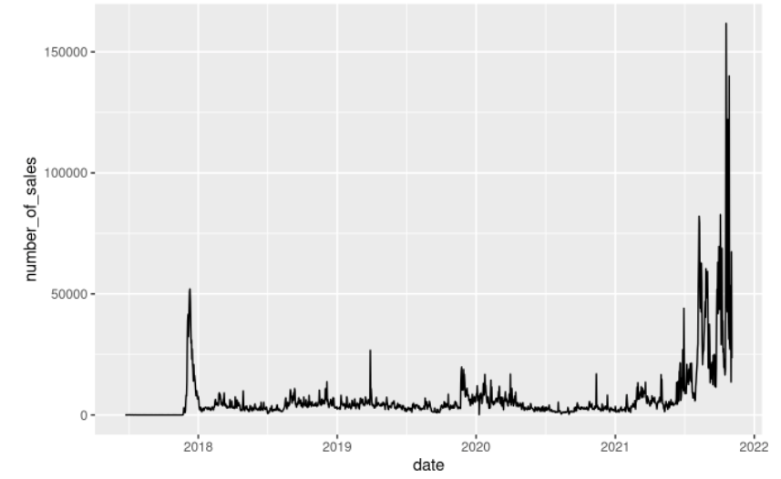
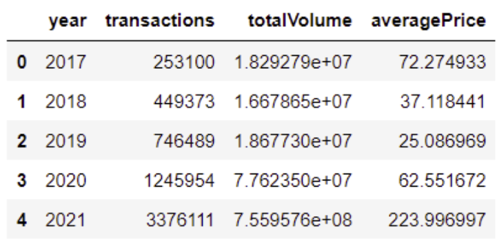
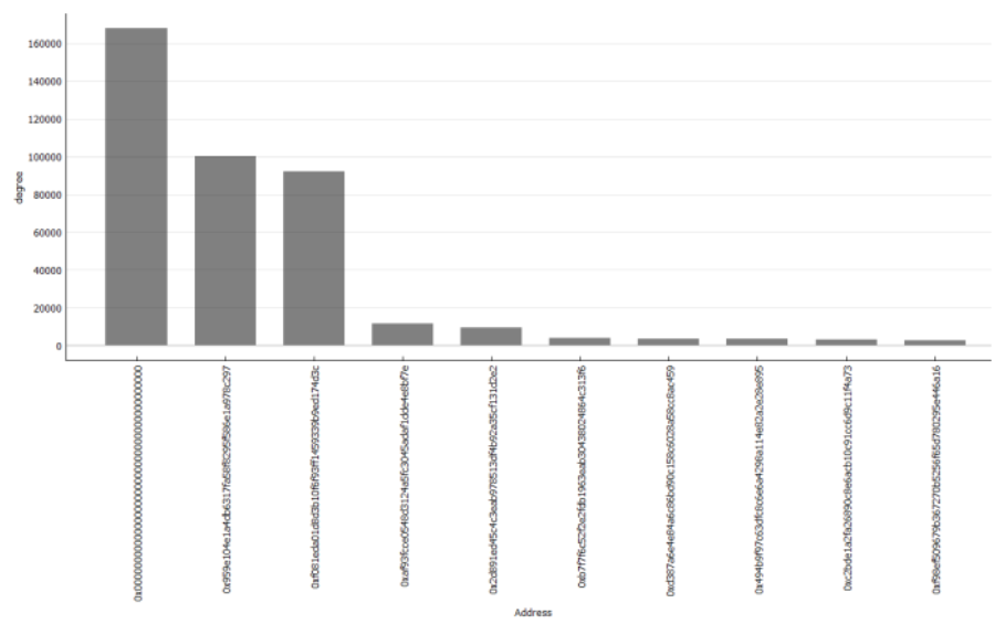
The sale of NFT skyrocketed in 2021; fig6 shows the average amount of sales over time. We can observe the table1 which shows the year's increase in the number of transactions. In 2018 there were only 450 thousand transactions, whereas in 2021, there we almost three and a half million transactions. If we look at table 1, we can see a boom in NFT world as in the first quarter only; the total volume has been rising to nearly 760 million USD. Here the indegree and outdegree of each node is too large to visualize; the fig7: shows the top 10 accounts that have high degree value. This high degree value means that these addresses are active in trading the NFTs. The highest number of NFT is, as shown in the fig7 is held under an address starting from 0x0000. This means that any user does not own this address; these addresses are associated with NFTs when they are the first minted.
We selected the major 7 NFT projects [37] of all time as per the number of sales over the period and calculated the semantics of the combined network by performing graph analysis on the transaction data. We observed that there was a total of 33678 unique addresses, which represent nodes of the graph, similarly 425246 number of transactions between those addresses.
The constructed network is a directed graph. We calculated the graph network reciprocity, associativity, connected component and k-core properties of the network. The reciprocity of a directed graph gets the likelihood of nodes in a directed network being mutually linked.

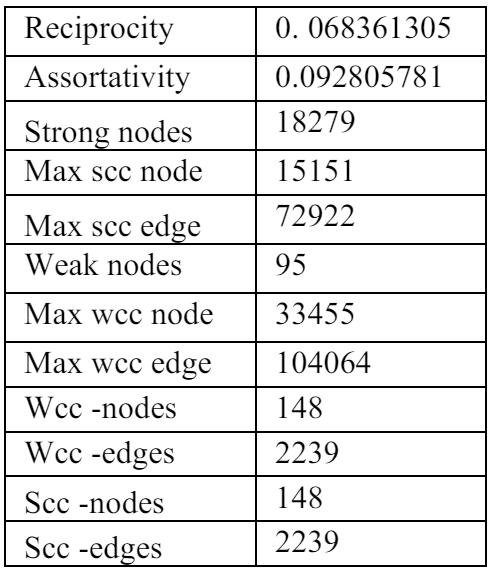
Here the ratio is the number of edges pointing in both directions to the total number of edges in the graph. This shows the trade transaction between the user nodes. Similarly, in the above equation. The reciprocity of a single node u is defined. It is the ratio of the number of edges in both directions to the total number of edges attached to node you. G denoted the directed graph. The reciprocity of the graph was observed to be 0.068361305. Similarly, we found out among the nodes, 18279 were strong nodes and 72922 strong, connected edges between the nodes, and we observed that the max weak nodes were 95 nodes only; this shows how well connected all the nodes are. We observe that the max weak connected components edges counts were 104064. Table 2 gives all other graph parameters that are observed from the NFT transaction graph. Table 2 shows strong, connected nodes and edges count. The assortativity is calculated in an indirection graph.
Here we first combined the 7 different CSV into a single collection and assigned each address a unique id. giant () method was used to get the strongly connected components, a similar approach for the weak components. Then we calculated the core from the large weakly connected components and used the k_core method to obtain the number of strong and weak connected component vertex and edge count.
The below figure shows the ALL NFT network component as shown here the buyer, and the seller are created from the trader, and the transaction is considered a component for better visualization.
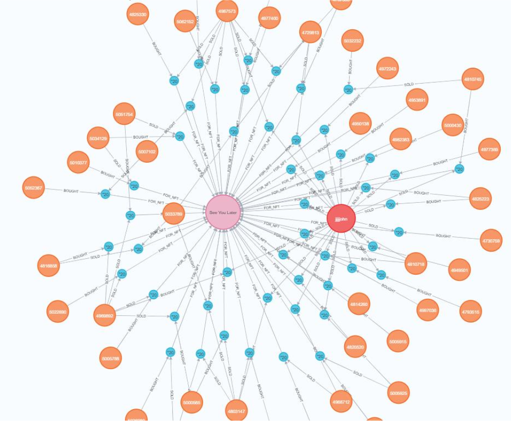
As shown in fig2. Let’s us take an example to visualize the transaction of a Single NFT transaction over the period. As we can see in the below figure. The pink color is an NFT called “See You later” and the red is the create of the NFT and then all the orange nodes are the buyer and seller from the time of creating the NFT. The blue color represents the transaction and the kind of transaction that happened. For example, it shows which wallet sold the NFT and which wallet bought the NFT from that transaction.
We can see the graph schema contains the collection components. Most of the popular NFT belong to a collection. We can see the example in real-world where most of the famous paintings of a famous artist are sold at high prices. In a similar manner, the collection of NFT and who created the NFT determines the worth of the NFT Collection. There is not any price limit as there is no condition on how much the price can be set.
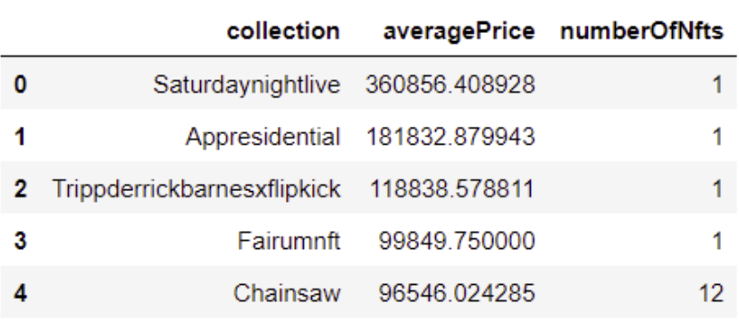
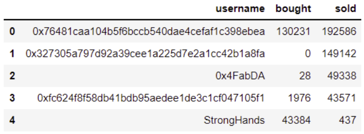
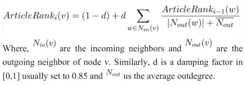
Similarly, to get furthermore InSite on to influence nodes in the NFT network, we used Article Rank algorithm, which is a variant of the PageRank algorithm. It measures the transitive influence of nodes.
Neo4j provides us with built in methods to calculate the ranking. Here the Article rank lowers the influence of low degree nodes by lowering the score being sent to their neighbor in each interaction.
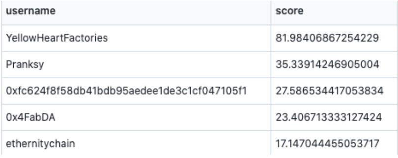
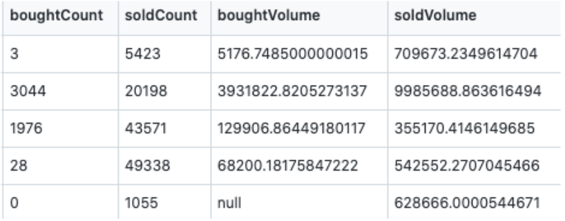
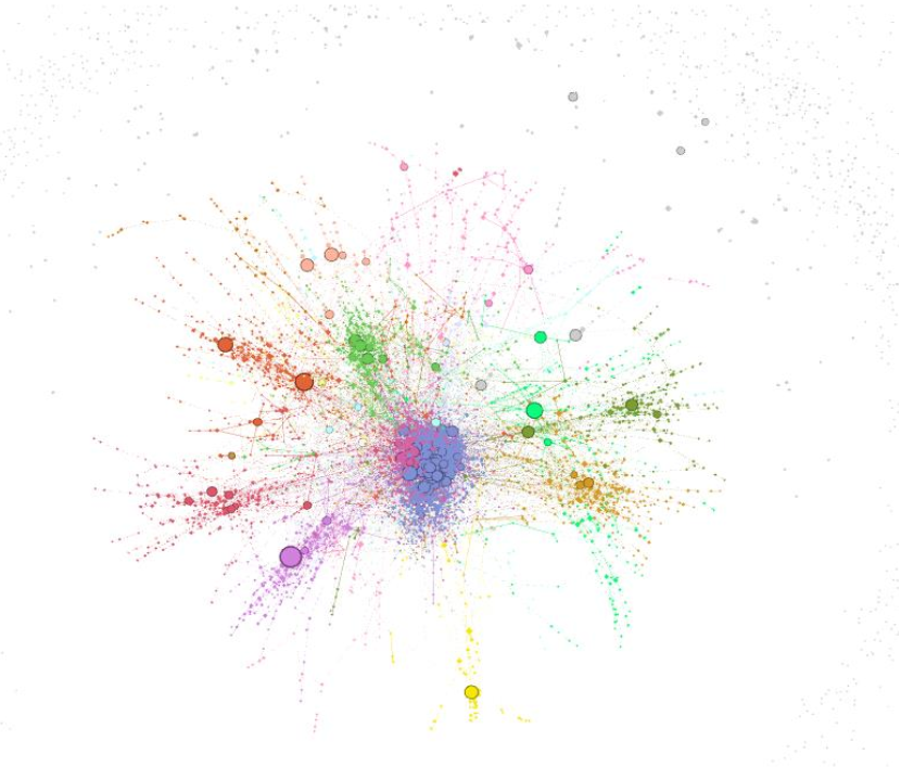
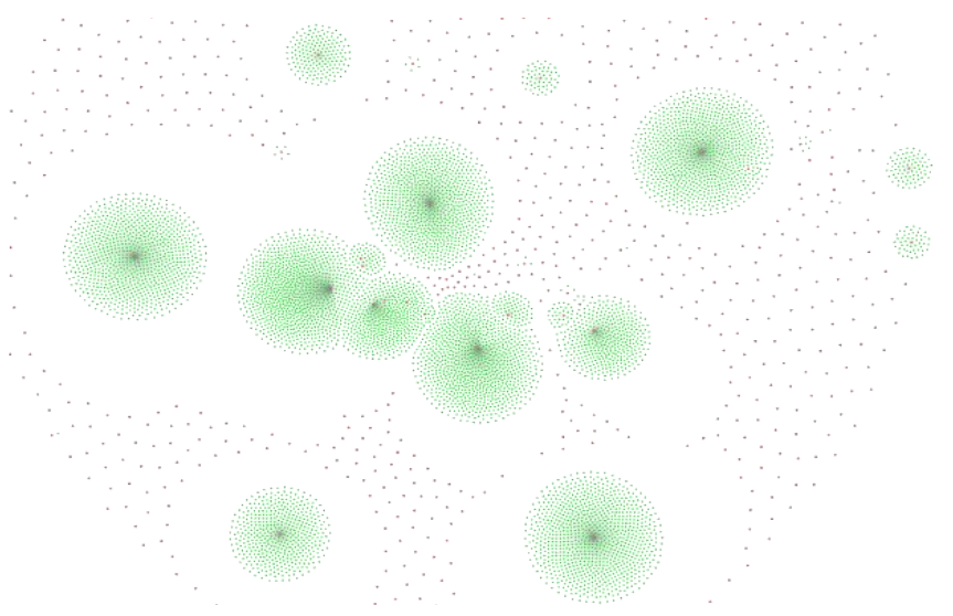
The Table 5 & 6 show the most influencer NFT collectors of the network and their trading value. The sold and bought volume is in USD. This shows there is signifying amount of transaction influence by these nodes. In the Fig 9 we can observe a community of such influence nodes distinct using a different color. We can observe a denser community at the center and multiple such high influence nodes and multiple small communities being formed around them and these nodes are densely connected signifying high transaction between the nodes.
This paper is available on arxiv under CC BY 4.0 DEED license.
