LPPL (Logarithmic Periodic Power Law) Model Effectively Predicts NFT Market Bubbles

Table of Links

Abstract and 1 Introduction

2 Related Works

3 Datasets and Experiment Setup

4 Methodology

4.1 NFTs Transaction Network

4.2 NFTs Bubble Prediction

5 Discussion and Conclusions, and References

4.2 NFTs Bubble Prediction

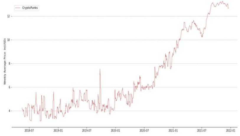
In recent years, the LPPL model[38] has been studied in different research for bubble detection, here, the model uses time-series price data. This model assumes the presence of two types of agents in the market: a group of traders with rational expectations and the second group of so-called “noise” traders, that is, irrational agents with herding behavior. The algorithm approximates the log price of the data at a given period t. as

where A, B and C are the linear parameters and other are the nonlinear parameters Tc, m, w, φ. In the above equation, Tc denotes the singularity at which the previous bubble ends and transitions to another set. A denotes the log price, B denotes the magnitude of the power law acceleration and ranges from B>0 for the increasing price to B<0 for decreasing price. The LPPL model derives these positive and negative bubble indicators to all t2, thereby visualizing its own predictions. Similarly, C denotes the magnitude of the logperiodic oscillations, where if m=1, C=0, then LPPL reduces to an exponential fit of the price time series. If m<1, then LPPL grows super-exponentially until the critical time T. If C, w>0, then LppL exhibits oscillation that becomes progressively more frequent as x approaches the critical time. Here for the model, we need to calibrate the model. Model calibration can be defined as finding a unique set of model parameters that provide a good description of the system behavior and can be achieved by confronting model predictions with actual measurements performed on the system. For our test the model is calibrated with the Ordinary Least square method, providing the estimations of all parameters mention in the above equation. Similarly, the equation also contains non-linear parameters. we set the following calibration for a given time [t1, t2]. We then make bubble predictions at each period of the data, by letting this calibration iterate for the shrinking time window [t1, t2].

According to the daily data, [t1, t2] is in daily units. t2 denotes a fictitious today corresponding to t; t1 denotes an earlier day. For a given t2, the iterative calibration sets the initial range of the time window as 120 days and the shrinking Interval of t1 as 5 days. That is, we need to estimate parameters 24 times for each t2 (e.g., [1, 120], [5, 120], …, [115, 120]). This process emphasizes the prediction and here we use only historical data as input. The outcome of t2 depends only on data from t2 to the last 120 days.